Traditional hardware addition

Trees calculate one digit of the answer. What calculates the whole thing?

The brief theory of addition notebook discussed the calculation of a single digit of the final answer. Such a calculation can be associated in numerous ways, each one representing a specific digital circuit. Combinatorics tells us that the space of possible associations of \(n\) factors is bijective with the space of possible binary trees of \(n\) leafs.

Subsequently though, how can the entire of the final multi-digit answer be represented, as opposed to just one of its digits?

Clasically, this is done through a tree with multiple roots, one for each digit. This structure is known as a polytree, or an \(n\)-rooted tree.

Classic structures

This section presents several classic adder structures.

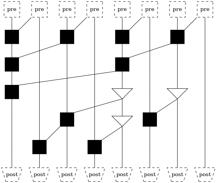
The diagrams shown below are drawn in the classic style of adder literature.

Data flows from top to bottom. Thus the \(n\) roots of the tree sit at the bottom. Nodes labeled “pre” perform pre-processing logic that encodes \(a\) and \(b\) into an alternate form. Nodes labeled “post” re-compose the local and non-local aspects of binary addition into the final sum. The main body of the diagrams performs the non-local computation.

Serial structure

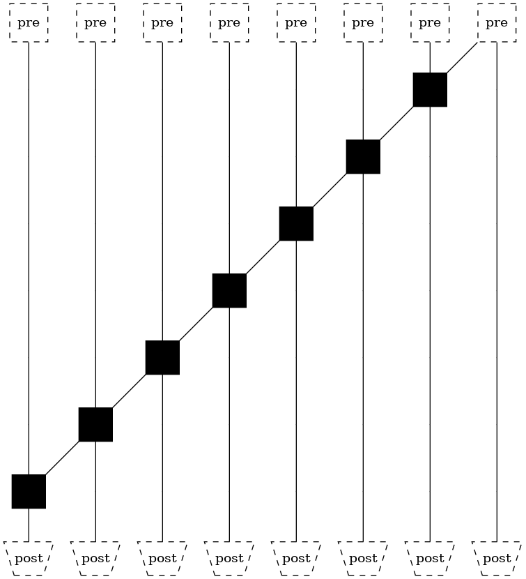
This is the naïve implementation of adding one digit at a time and “carrying over the one”.

Sklansky structure

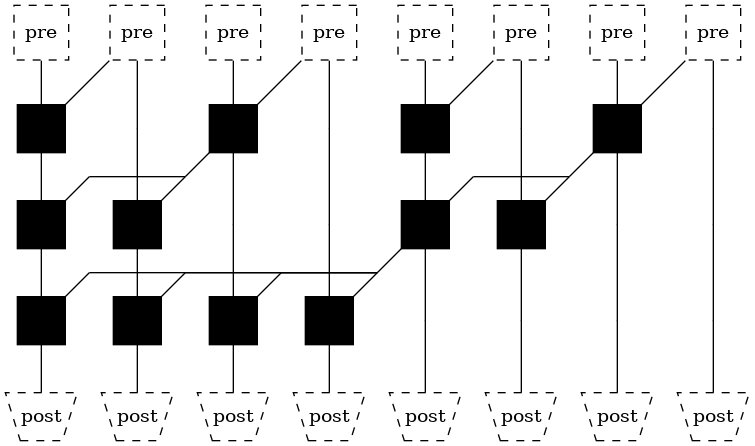
This is a right-balanced \(n\)-rooted tree.

The height of the tree (the number of sequential logic levels) has dropped from \(n-1\) to \(lg(n)\), thus decreasing the delay.

The number of nodes has risen, thus increasing both area and power consumption.

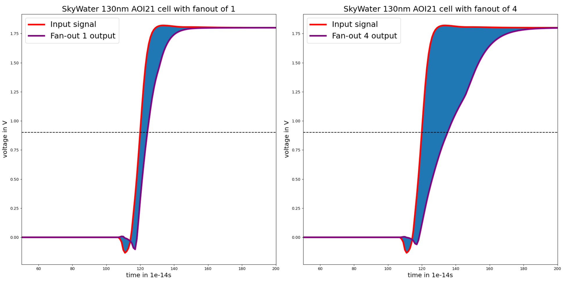
However, it may be observed that some nodes drive multiple outputs. This is a concept known as fanout. Fanout directly increases delay. as can be seen from the simulation results below.

Kogge-Stone structure

This is a left-balanced \(n\)-rooted tree.

It can be seen to have minimal fanout. As such, it should be faster than the previous structure.

The height of the tree (the number of sequential logic levels) remains at \(lg(n)\), thus decreasing the delay.

The number of nodes has risen, thus increasing both area and power consumption.

However, it may be observed that some of the gaps between the rows of nodes have multiple sets of parallel wires running through them. This concept is known as wire tracks. An increased need for wire tracks also directly increases the delay. Either the wires are placed in close proximity, and cross-coupling capacitance degrades performance, or the wires are spaced out, and the electrical signal has to deal with longer wires.

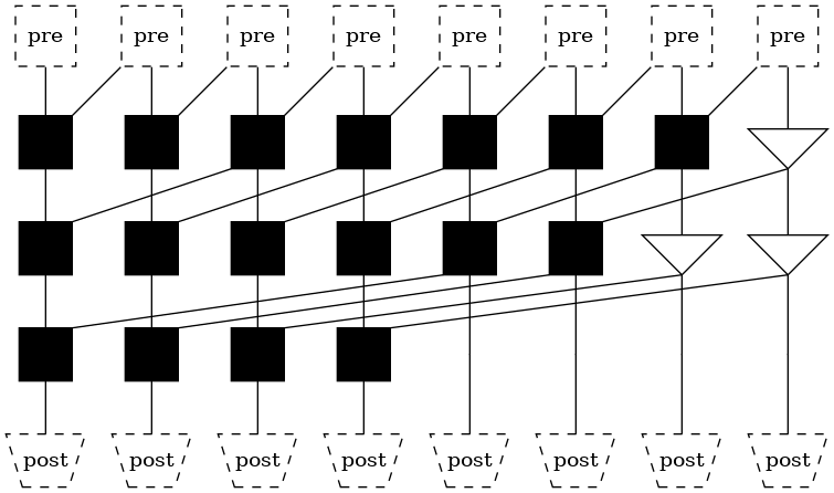
Brent-Kung structure

This is a tree with both minimal fanout as well as minimum wire tracks.

However, the number of logic levels is higher than both previous examples, at \(2lg(n)-1\).

Trade-offs (layers, fan-out, tracks)

The brief theory of addition notebook discussed the question “Why is this huge design space relevant at all?” These necessary trade-offs, between layers, fan-out, and tracks, is why the design space must be explored.

While both the Sklansky and Kogge-Stone structures are balanced, their fan-out and tracks reduce their actual speed in physical implementation. The fastest structure is often neither of them, but rather a compromise.

Furthermore, each of these structures incurs a large cost of area and power consumption. The Brent-Kung structure, for example, still has logarithmic delay, but consumes far less power.

Another important point is that these circuits generate multiple output bits. In practice, not all these output bits are equally important. Exploring the design space allows for the creation of custom structures that are optimal for non-uniform timing constraints.

Problems with classic hardware addition

As previously mentioned, classic addition theory chooses to represent the calculation of an \(n\)-bit binary addition as an \(n\)-rooted tree in the form of the above diagrams.

There are several key flaws with this reasoning:

• The inputs and outputs are strangely offset by 1, requiring alien notation such as “the negative first bit of the input”.

• The design space is restricted by assumptions such as “only one node may occupy a certain location in the diagram” or “each node must be connected to the node above it”. These are unnecessary assumptions that eliminate useful architectures.

• It is entirely unclear what the pre-processing logic does, how it relates to the rest of the tree, and how this can be used to optimize addition.

• It is entirely unclear what the post-processing logic does, how it relates to the rest of the tree, and how this can be used to optimize addition.

Revised hardware addition

Setup (RUN ME before executing any code in this section)

!pip install --upgrade git+https://github.com/tdene/synth_opt_adders.git@v1.0.8

Defaulting to user installation because normal site-packages is not writeable
Collecting git+https://github.com/tdene/synth_opt_adders.git@v1.0.8
  Cloning https://github.com/tdene/synth_opt_adders.git (to revision v1.0.8) to /tmp/pip-req-build-62j3w7e4
  Running command git clone --filter=blob:none --quiet https://github.com/tdene/synth_opt_adders.git /tmp/pip-req-build-62j3w7e4
  Running command git checkout -q b7fefb354f08171a8d9cd6e623d9b83c9d77581a
  Resolved https://github.com/tdene/synth_opt_adders.git to commit b7fefb354f08171a8d9cd6e623d9b83c9d77581a
  Preparing metadata (setup.py) ... done
Requirement already satisfied: Pillow in /home/tdene/.local/lib/python3.8/site-packages (from pptrees==1.0.8) (9.1.1)
Requirement already satisfied: graphviz in /home/tdene/.local/lib/python3.8/site-packages (from pptrees==1.0.8) (0.19.1)
Requirement already satisfied: networkx in /home/tdene/.local/lib/python3.8/site-packages (from pptrees==1.0.8) (2.7)
Requirement already satisfied: pydot in /home/tdene/.local/lib/python3.8/site-packages (from pptrees==1.0.8) (1.4.2)
Requirement already satisfied: pyparsing>=2.1.4 in /home/tdene/.local/lib/python3.8/site-packages (from pydot->pptrees==1.0.8) (3.0.7)
Building wheels for collected packages: pptrees
  Building wheel for pptrees (setup.py) ... done
  Created wheel for pptrees: filename=pptrees-1.0.8-py3-none-any.whl size=63945 sha256=b88c75060dabcd09e91db472fa04f36da87c3b99ea50685dadde0e59ec746f7d
  Stored in directory: /tmp/pip-ephem-wheel-cache-921bsjmq/wheels/6a/0e/65/6c50e0a68c52fea65d7c9d6ba6a57e5a84e3d619b2357f716d
Successfully built pptrees
Installing collected packages: pptrees
Successfully installed pptrees-1.0.8
WARNING: You are using pip version 22.0.4; however, version 22.1.2 is available.
You should consider upgrading via the '/usr/bin/python3 -m pip install --upgrade pip' command.

from pptrees.AdderTree import AdderTree as tree
from pptrees.AdderForest import AdderForest as forest
from pptrees.util import catalan

Trees calculate one digit of the answer. What calculates the whole thing?

A circuit that calculates a single digit of the final answer is analogous to a binary tree.

Classic addition theory chooses to represent the calculation of an \(n\)-bit binary addition as an \(n\)-rooted tree in the form of specific diagrams.

Let’s instead represent \(n\)-bit binary addition as a non-disjoint forest of \(n\) trees.

The classic structures

Here are the classic structures from the previous section, in this representation.

from pptrees.AdderForest import AdderForest as forest

# Serial structure
f = forest(9)
f

from pptrees.AdderForest import AdderForest as forest

# Sklansky structure
f = forest(9)
for t in f.trees[2:]:
  t.rbalance(t.root[1])
f

from pptrees.AdderForest import AdderForest as forest

# Kogge-Stone structure
f = forest(9)
for t in f.trees[2:]:
  t.lbalance(t.root[1])
  t.equalize_depths(t.root[1])
f

from pptrees.AdderForest import AdderForest as forest

# Brent-Kung structure, before the fan-out is decoupled
f = forest(9)
for t in f.trees[2:]:
  t.rbalance(t.root[1])
  # Same as Sklansky so far
  while not t.root[1][0].is_proper():
    t.right_rotate(t.root[1][0])
f

from pptrees.AdderForest import AdderForest as forest

# Brent-Kung structure, before the fan-out is decoupled
f = forest(9)
for t in f.trees[2:]:
  t.rbalance(t.root[1])
  # Same as Sklansky so far
  while not t.root[1][0].is_proper():
    t.right_rotate(t.root[1][0])

# And now Brent-Kung with the fan-out decoupled
f.calculate_fanout()
f.decouple_all_fanout(2)
f.unmark_equivalent_nodes()
f

These all generate the same hardware as the structures in the previous section.

Post-classic structures

Here are some examples of structures that are impossible to depict under the old system.

First, it is now known exactly how many possible structures there are.

Note that architectures that differ only in the method of decoupling their fanout are considered fundamentally equivalent. Buffer insertion, or fanout decoupling, is not an inherent feature of logically synthesized hardware. It is a layout optimization to be performed after logical synthesis.

width = 9
number_of_structures = 1
for a in range(2,width):
  number_of_structures = number_of_structures * catalan(a-2)
print(number_of_structures)

776160

Here is one arbitrary structure that is impossible to depict, generate, or describe using traditional methods.

f = forest(9, tree_start_points = [0, 0, 0, 1, 4, 12, 21, 47, 217])
f

There are many such examples. The notebook on sparseness and the notebook on factorization introduce two important concepts that are poorly understood and under-utilized due to the traditional method of regarding arithmetic circuits.