Brief theory of addition¶

Importance¶

Binary addition is one of the most used and important operations in computing. For example, when booting a RISC-V processor into Linux over 2/3rds of the assembly instructions will use addition in some manner.

Circuit design involves trade-offs, typically phrased in terms of power vs performance (speed) vs area. Circuits can be very fast and power-hungry, very slow and power-efficient, or anywhere in between.

Moreso, these trade-offs occur on a bit-by-bit basis. If a circuit generates a 64-bit result, each bit of the result can be optimized for power, speed, or area. Often this becomes essential, as some bits must be processed faster than others.

Thus, optimizing adder hardware affects entire designs.

Breakdown of addition¶

Binary addition has a “local” and “non-local” component. A proper explanation of this concept involves exact sequences and cohomology groups. Fortunately for you, I am not familiar enough with that math to bore you with a technical explanation.

Take the following example:

999 +
001
  _______
000 000

Each digit of the sum depends “locally” on the corresponding digits of each input. But all digits of the sum also depend “non-locally” on all digits to the right. The $1$ on the far right affects even the left-most digit of the result. It is impossible for a general circuit to compute the correct answer without accounting for that $1$.

In math terms, for $s = a+b$, the digit $s_i$ depends locally on $a_i$ and $b_i$, and non-locally on all $a_j, b_j$ where $i > j$.

The local aspect of binary addition can be resolved in parallel, in a single time-step, for every digit. Again, $s_i$ depends locally only on $a_i$ and $b_i$. For an $n$-bit adder, just instantiate $n$ copies of the hardware, and process all bits of $a$ and $b$ at the same time.

The non-local aspect is more complex. This is what is known as the “carry”. Overflow from one pair of digits may affect the next pair of digits. The naïve grade-school implementation of adding one digit at a time and “carrying over the one” uses $n$ time-steps. Speeding it up by doing two digits at a time can reduce that to $n/2$ time-steps, but that’s still O(n).

O(n) is very slow. O(lg n) on the other hand is both fast and achievable.

Brief theory of arithmetic operations¶

Arithmetic computation in logarithmic time¶

An extensive body of literature provides a three-step recipe for speeding up non-local aspects of a computation.

Express the non-local computation of digit $i$ as $Y_i = X_i ■ Y_{i-1} $. $Y$ is the output, $X$ is the input, $■$ is some pre-determined operator.
Expand: $Y_i = X_i ■ X_{i-1} ■ X_{i-2} ■ \dots X_0$. Clearly this is a non-local computation: every output depends on all previous inputs, in some manner that is determined by $■$.
Associate: $Y_i = (X_i ■ X_{i-1}) ■ (X_{i-2} ■ \dots X_0)$

The expression in step #2 takes $i-1$ steps. The expression in step #3 can take anywhere from $lg(i)$ to $i-1$ steps, depending on how association is performed.

For a concrete example, compare the following 7-step operation:

$Y_7 = X_7 ■ (X_6 ■ (X_5 ■ (X_4 ■ (X_3 ■ (X_2 ■ (X_1 ■ X_0))))))$

To a 3-step alternative:

$Y_7 = (((X_7 ■ X_6) ■ (X_5 ■ X_4)) ■ ((X_3 ■ X_2) ■ (X_1 ■ X_0)))$

The first formula performs all operations sequentially. The second formula is parallelized, and MUCH faster.

How many ways can you associate an expression?¶

An expression of $n$ terms such as the one above can be associated in $C_n$ ways, where $C$ represents the Catalan numbers.

What else do the Catalan numbers represent? The number of ways different ways to draw a binary tree with $n+1$ leafs.

That means that all such arithmetic circuits can be mapped to and from binary trees.

See the binary tree space traversal notebook for further discussion.

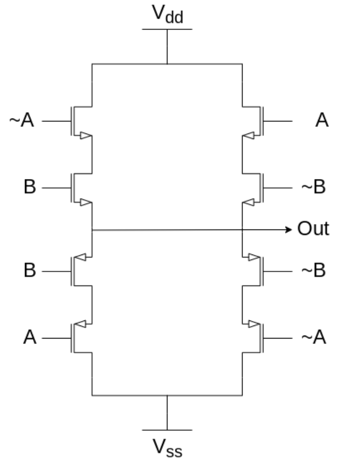
What is ■?¶

There’s a simple recipe to determine ■ for any arithmetic operation. It is further discussed in the general operation theory notebook.

Here is ■ for addition, shown as a CMOS logic schematic:

Why is this huge design space relevant at all?¶

In software, a balanced tree with $lg(n)$ height is often optimal. In hardware, the sacrifices needed to balance a tree to $lg(n)$ height can outweigh the benefits. Sometimes it is actually faster to use a circuit that performs more sequential operations back-to-back.

Key concepts that hardware, unlike software, must account for are fan-out (given an output, how many inputs does it connect to?) and cross-coupling capacitance (parallel wires carrying electrical signals will mutually degrade each others’ performance). Both of these effects will severely degrade a circuit’s performance, turning what would otherwise be an easy design choice into a complex design space.

Meanwhile, a concept that hardware and software share in-common is the trade-off between time complexity and space complexity. Let us say that a software engineer is given the choice between a software algorithm with O(n) time complexity and O(n) space complexity, and an algorithm with O(lg n) time complexity and O(n lg(n)) space complexity. The sofware engineer may give it some thought, but ultimately the choice doesn’t matter very much on modern hardware.

For a hardware engineer though, the difference between O(n) space complexity and O(n lg(n)) space complexity may be the difference between a working chip and a useless space heater.

This is illustrated in more detail in the notebook comparing traditional hardware addition to revised hardware addition.

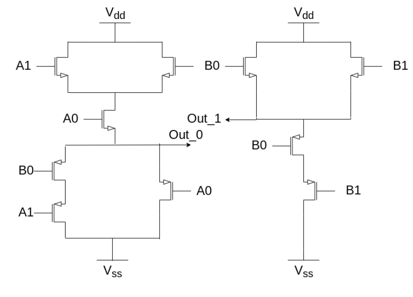
Wait, what about the local component??¶

The local component of any arithmetic operation can also be determined from a simple recipe.

It is less interesting than the non-local component. Fully parallelizing it is trivial: simply instantiate $n$ copies of the hardware and perform all the local computations in parallel in a single time-step.

Typically the local component is calculated separately, then combined with the non-local component at the very end of the operation to yield the final result.

Here is the local component for addition, expressed as a CMOS logic schematic.

Once both the local and non-local components have been computed, they are combined to obtain the final answer.

In general, this final composition takes the form of an if-then statement (some fashion of multiplexer gate).

For addition in particular, this final composition happens to use the same type of gate as the one seen above.